Using BMS to reproduce the body fat example from "Bayesian Model Averaging: A Tutorial" (1999)

In their paper Bayesian Model Averaging: A Tutorial (Statistical Science 14(4), 1999, pp. 382-401), Hoeting, Madigan, Raftery and Volinsky (HMRV) do an exercise in Bayesian Model Averaging (BMA) at pp.394-397 in estimating body fat data from Johnson (1996): "Fitting Percentage of Body Fat to Simple Body Measurements"; Journal of Statistics Education 4(1).
This tutorial shows how to reproduce the results with the R-package BMS.

Getting R and BMS

Before continuing with the tutorial, you should have R installed (any version > 2.5) and the library BMS installed.

How HMRV Did It

The following is a short outline of how FLS set up their BMA example on pp.394-397:

They use data from Johnson (1996) with 13 covariates and 251 observations. (The original data contains 252 observations, but one is omitted.)
HMRV use slightly different priors compared to BMS:
- HMRV use proper priors on variance and the intercept, that differ slightly from the standard framework used in BMS.
- Prior coefficient covariance: They do not rely on Zellner's g prior as does BMS, but instead use a diagonal matrix: However, their matrix is the same as under Zellner's g prior, with the off-diagonal elements set to zero.
- Consequently, HMRV use a notation that differs from the approach used in Zellner. But since the coefficient prior nearly coincides, Zellner's g in BMS is equivalent to their choice of phi^2*n. Since they choose phi=2.85 the equivalent g-prior should be approximately 2000.
Their model prior is the uniform model prior (same prior probability for all models) - (p.7).
For sampling through the model space, they use complete enumeration of all models.
They base their final posterior model probabilities on the analytical posterior model probabilities of all models.

Getting the Body Fat Data

The original data is available from the web appendix of Johnson (1996) as the file fat.dat
Before downloading it, find out your current working directory by opening R and typing the following into the R console:

getwd()

Download fat.dat to this location. Then load it into R by

fat1=read.table("fat.dat")

fat1 becomes a data.frame containing the data. HMRV take only a meaningful sub-sample of these. A glance at fat.txt reveals which data they are.
Therefore the next step is to consolidate fat1 to the same data as used in HMRV, by extracting the response variable (column 2) and the explanatory variables from HMRV (columns 5-7 and 10-19).

fat = fat1[,c(2, 5:7, 10:19)]

Moreover, HMRV drop observation 42 since its reported body height is only 29.5 inch (75 cm). Finally, let's assign more meaningful names to the data.

names(fat)=c("brozek_fat","age","weight","height","neck","chest","abdomen","hip","thigh","knee","ankle","biceps","forearm","wrist")
fat= fat[-42,]

Replicating: Demonstration

First, load the package BMS with the following command

library(BMS)

Now we can sample models according to HMRV: We need a fixed g prior equal to 2000 - set by the argument g=2000. The model priors should be uniform and are assigned via mprior="uniform". Finally, mcmc="enumeration" requires full enumeration of all models and should be quite fast: 2^13=8192 potential models, which should take two to three seconds to compute.

mf= bms(fat,mprior="unif",g=1700, mcmc="enumeration", user.int=FALSE)

The variable mf now holds the BMA results and can be used for further inference. The argument user.int=FALSE just suppresses printing output on the console in order to avoid confusion in this tutorial.
HMRV report standardized coefficients in Table 8. This can be reproduced by typing:

coef(mf,std.coefs=TRUE)

Here, std.coefs=TRUE forces the coefficients to be standardized (as if for data with mean zero and variance one). The above command produces the following output

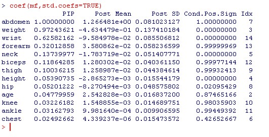
The first column PIP above holds the posterior inclusion probabilities that correspond to the fifth column in Table 8 of HMRV (p.396). The values match up pretty well, even though the prior concept used here was different from HMRV.
The column Post Mean reports posterior expected values of coefficients ('Mean' in HMRV Table 8) which are, again quite close to the ones in the article. The same applies to their standard deviations (PostSD). The slight differences are most likely due to the effect exerted by Zellner's g prior vs the prior used by HMRV.
Note that the coefficients in HMRV are also sign-standardized (no negative signs), which is not the case here.

The Other Results

In addition to PIPs and coefficients, HMRV report a graphic representation of the best 10 models (by posterior model probability) in their Table 9.
The BMS equivalent can be plotted with the following command:

image(mf[1:10],order=FALSE)

The [1:10] means that only the best ten models should be plotted (for more on best models consider argument nmodel in help(bms)). order=FALSE orders the output according to the original data.
The output looks as follows - note that only the variables included among the top ten models are shown, just as in HMRV, Table 9:

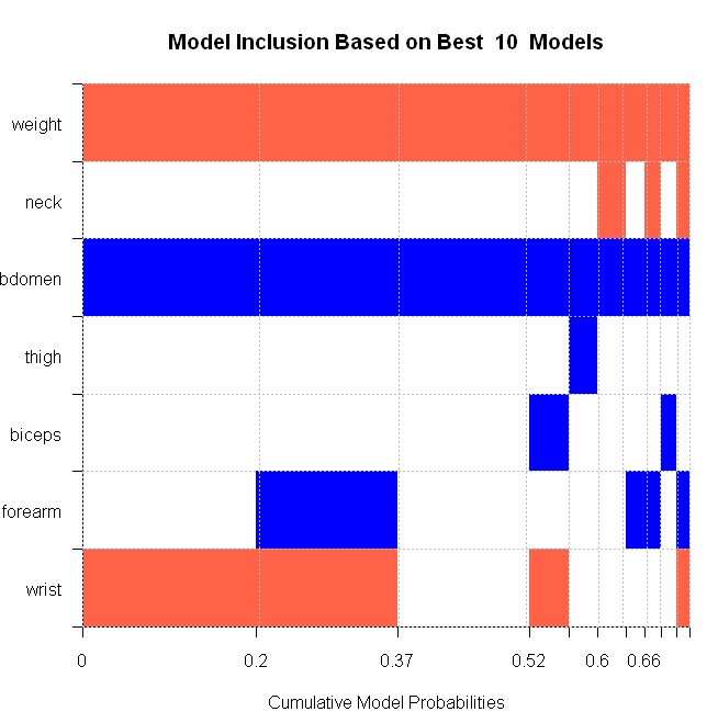
The chart can be read as follows: The very best model is plotted to the left-hand side, and contains three variables: weight (red for negative sign), abdomen (blue for positive coefficient) and wrist (red for negative). This best model has a posterior model probability of 20%. To its right is the second-best model, which contains forearm in addition. The other models follow.
In its structure, this image conforms to Table 9 in HMRV. However, the reported posterior model probabilities are different in absolute values, which is due to the different prior structures employed. Nonetheless, the model distribution corresponds to HMRV in relative magnitudes.

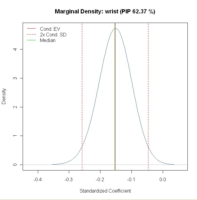
Finally, HMRV report the posterior density for the standardized coefficient of wrist in Figure 4. Replicate this plot with the following command:

density(mf,reg="wrist",std.coefs=TRUE)

The result looks exactly similar to Figure 4 in HMRV:

More Results

There are several other functions in the BMS package that can be used to explore the data further. Try out the following commands:

plotModelsize(mf) plots the prior and posterior model size distribution
summary(mf) reports some summary statistics, in particular posterior expected model size.
help(bms) reveals more about the prior options to play around with body fat data.
Refer to the documentation for even more functions.